Analysis of Biden approval margin


# Bidens Approval Margins

As we saw in class, fivethirtyeight.com has detailed data on [all polls that track the president's approval ](https://projects.fivethirtyeight.com/biden-approval-ratings)


```r
# Import approval polls data directly off fivethirtyeight website
approval_pollist <- read_csv('https://projects.fivethirtyeight.com/biden-approval-data/approval_polllist.csv') 

glimpse(approval_pollist)

## Rows: 1,600
## Columns: 22
## $ president           <chr> "Joseph R. Biden Jr.", "Joseph R. Biden Jr.", "Jos~
## $ subgroup            <chr> "All polls", "All polls", "All polls", "All polls"~
## $ modeldate           <chr> "9/17/2021", "9/17/2021", "9/17/2021", "9/17/2021"~
## $ startdate           <chr> "1/31/2021", "2/1/2021", "2/1/2021", "2/2/2021", "~
## $ enddate             <chr> "2/2/2021", "2/3/2021", "2/3/2021", "2/4/2021", "2~
## $ pollster            <chr> "YouGov", "Rasmussen Reports/Pulse Opinion Researc~
## $ grade               <chr> "B+", "B", "B", "B", "B", "B-", "A-", "B", "B-", "~
## $ samplesize          <dbl> 1500, 1500, 15000, 1500, 15000, 1005, 1429, 15000,~
## $ population          <chr> "a", "lv", "a", "lv", "a", "a", "a", "a", "rv", "l~
## $ weight              <dbl> 1.0856, 0.3308, 0.2786, 0.3086, 0.2507, 0.8741, 2.~
## $ influence           <dbl> 0, 0, 0, 0, 0, 0, 0, 0, 0, 0, 0, 0, 0, 0, 0, 0, 0,~
## $ approve             <dbl> 46, 52, 54, 49, 54, 57, 49, 54, 60, 50, 54, 55, 51~
## $ disapprove          <dbl> 38, 46, 33, 48, 34, 34, 39, 34, 32, 47, 34, 33, 46~
## $ adjusted_approve    <dbl> 47.2, 54.4, 52.5, 51.4, 52.5, 55.9, 49.6, 52.5, 59~
## $ adjusted_disapprove <dbl> 38.3, 40.1, 36.3, 42.1, 37.3, 35.1, 39.1, 37.3, 33~
## $ multiversions       <chr> NA, NA, NA, NA, NA, NA, NA, NA, NA, NA, NA, NA, NA~
## $ tracking            <lgl> NA, TRUE, TRUE, TRUE, TRUE, NA, NA, TRUE, NA, TRUE~
## $ url                 <chr> "https://docs.cdn.yougov.com/460mactkmh/econTabRep~
## $ poll_id             <dbl> 74332, 74338, 74366, 74347, 74367, 74345, 74348, 7~
## $ question_id         <dbl> 139593, 139642, 139733, 139654, 139734, 139652, 13~
## $ createddate         <chr> "2/3/2021", "2/4/2021", "2/11/2021", "2/5/2021", "~
## $ timestamp           <chr> "13:01:54 17 Sep 2021", "13:01:54 17 Sep 2021", "1~

# Use `lubridate` to fix dates, as they are given as characters.
approval_pollist <- approval_pollist %>% 
  mutate(modeldate = lubridate::mdy(modeldate), 
         startdate = lubridate::mdy(startdate), 
          enddate = lubridate::mdy(enddate), 
          createddate = lubridate::mdy(createddate))

Create a plot

What I would like you to do is to calculate the average net approval rate (approve- disapprove) for each week since he got into office. I want you plot the net approval, along with its 95% confidence interval. There are various dates given for each poll, please use enddate, i.e., the date the poll ended.

# Create confidence levels
approval_margins <- approval_pollist %>%
  
  #Select enddate
  filter(!is.na(enddate)) %>%
  mutate(week=isoweek(enddate),
         margin=approve-disapprove) %>%
  
  #Group the data
  group_by(week, subgroup) %>%
  
  #Summarize data (use se formula for differences)
  summarise(
    mean=mean(margin), 
    sd=sd(margin), 
    count=n(), 
    se=sd/sqrt(count), 
    t_critical=qt(0.975, count-1), 
    lower=mean-t_critical*se, 
    upper=mean+t_critical*se)

glimpse(approval_margins)

## Rows: 99
## Columns: 9
## Groups: week [33]
## $ week       <dbl> 5, 5, 5, 6, 6, 6, 7, 7, 7, 8, 8, 8, 9, 9, 9, 10, 10, 10, 11~
## $ subgroup   <chr> "Adults", "All polls", "Voters", "Adults", "All polls", "Vo~
## $ mean       <dbl> 18.00, 15.85, 12.00, 20.72, 16.82, 10.89, 19.81, 15.98, 13.~
## $ sd         <dbl> 5.68, 8.94, 11.33, 4.37, 7.70, 6.90, 2.31, 7.60, 9.16, 3.71~
## $ count      <int> 8, 13, 6, 12, 19, 9, 13, 25, 14, 13, 26, 15, 13, 22, 11, 14~
## $ se         <dbl> 2.009, 2.480, 4.626, 1.261, 1.766, 2.300, 0.639, 1.520, 2.4~
## $ t_critical <dbl> 2.36, 2.18, 2.57, 2.20, 2.10, 2.31, 2.18, 2.06, 2.16, 2.18,~
## $ lower      <dbl> 13.250, 10.442, 0.108, 17.942, 13.110, 5.585, 18.415, 12.84~
## $ upper      <dbl> 22.8, 21.3, 23.9, 23.5, 20.5, 16.2, 21.2, 19.1, 18.3, 19.6,~

#Create the graph
approval_margins %>% 
  filter(subgroup == "Voters") %>%
  ggplot(aes(x=week, y=mean)) +
  
  #Set colors 
  geom_point(color="chocolate2", size=1.5) +
  geom_line(color="chocolate2")+
  
  #Add fill between lines
  geom_ribbon(aes(ymin=lower, ymax=upper),
              color="chocolate2", 
              fill="grey87", 
              linetype=1, 
              alpha=0.5, 
              size=0.3) +
  
  #Change limits, theme, scale, facet wrap and add fitted line 
  ylim(c(-15,50)) +
  theme_bw() +
  scale_x_continuous(breaks=seq(0, 35, 13))+
  scale_y_continuous(breaks=seq(-15, 10, 2.5))+
  geom_smooth(se=FALSE) +
  
  #Add horizontal line 
  geom_hline(yintercept=0, 
             linetype="solid",
             color = "chocolate2", 
             size=2) +
  
  #Add labels 
  labs( title="Estimating Approval Margins (approve-disapprove) for Joe Biden",
        subtitle = "Weekly average of all polls",
        x = "Week of the year",
        y = "Average Approval Margin (Approve - Disapprove)") +
  NULL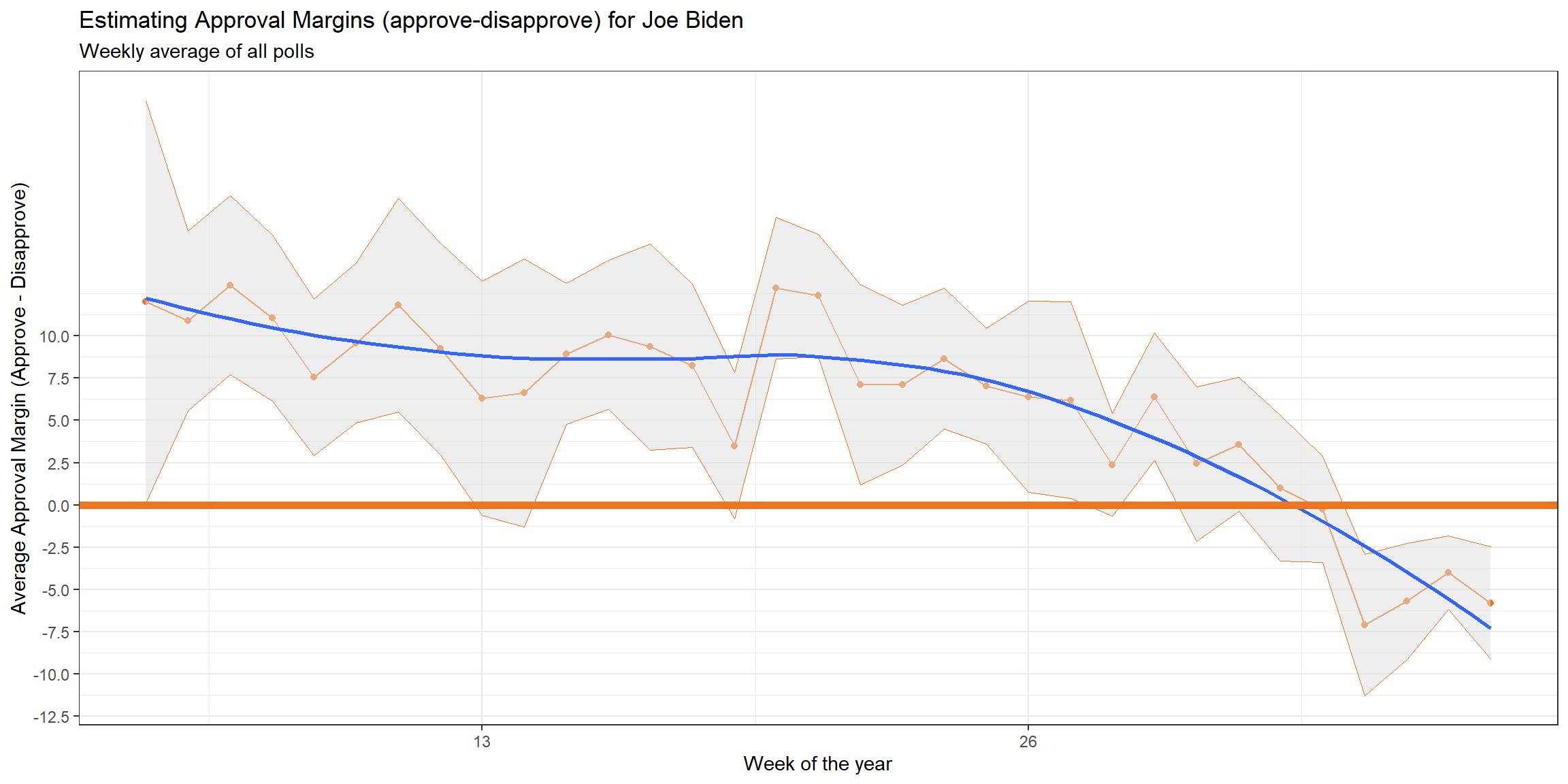

Compare Confidence Intervals

Compare the confidence intervals for week 4 and week 25. Can you explain what’s going on? One paragraph would be enough.

The sample set differs between week 4 and week 25. The sample size on week 3 is much smaller than that of week 25 which is why the standard error is relatively higher in week 3. This leads to larger confidence intervals in week 3 compared to week 25. As far as the data across the weeks is concerened, as sample size increases - confidence intervals shrink. The approval ratings for Joe Biden have reduced between week 4 and 25.